One Must Imagine Vlorbik Happy
Exam II is in a couple days. Zeros of polynomials, graphs of rational functions, compositions and inverses.
(I have just named three topics, not four; here [shrink the window to the size of a column] are some remarks on “the serial comma” I made back in th’ XXth c.)
Of course my classes are ill-prepared for this material, for the usual reason (no time to do things right). So I intend to look at some stuff that didn’t fit… but really to “review” work we’ve done along the way.
At the end of last week—very likely my most productive ever as a blogger, by the way—I mentioned that by applying the Transformations from the early part of the course—shifts and scalings—to the simplest Rational Function worthy of the name—of course I refer to the reciprocal function ![[x\mapsto {1\over x}]](https://s0.wp.com/latex.php?latex=%5Bx%5Cmapsto+%7B1%5Cover+x%7D%5D&bg=ffffff&fg=444444&s=0&c=20201002)

I used 


LF![:= \{ [x\mapsto {{Ax + B}\over{Cx + D}}] | A, B, C, D \in {\Bbb R} ; C \not= 0; AD-BC\not= 0 \}](https://s0.wp.com/latex.php?latex=%3A%3D+%5C%7B+%5Bx%5Cmapsto+%7B%7BAx+%2B+B%7D%5Cover%7BCx+%2B+D%7D%7D%5D+%7C+A%2C+B%2C+C%2C+D+%5Cin+%7B%5CBbb+R%7D+%3B+C+%5Cnot%3D+0%3B+AD-BC%5Cnot%3D+0+%5C%7D&bg=ffffff&fg=444444&s=0&c=20201002)
The inequalities at the end of this code exclude the cases where C is zero (which would give linear functions; this is easy to see) and where AD-BC is zero (which gives constant functions since then the numerator is a constant multiple of the denominator; this requires a small calculation to see).
Now. I sure haven’t proved that we’ll get this set by applying shifts and scalings to the reciprocal function. And ideally, this would be an exercise. For the course I happen to be running three sections of at this time, that would be absurd, however, so the next best thing would be to have it in the lecture notes. Which, while perfectly do-able in principle, appears unlikely. So here it is in the blog.
The general shifting-and-scaling Transformation (on 

![[ (x, y) \mapsto (Wx + H, Ay + K) ]](https://s0.wp.com/latex.php?latex=%5B+%28x%2C+y%29+%5Cmapsto+%28Wx+%2B+H%2C+Ay+%2B+K%29+%5D&bg=ffffff&fg=444444&s=0&c=20201002)

Probably no teacher of this material could now resist the temptation to point out what is presumably obvious to any actual reader of these notes: in the “f-notation”, one has a subtraction and a division where unguided “common sense” might lead the unwary to expect a multiplication and an addition. Anyhow, I can’t. Let’s go. The lecture I’m imagining would then begin.

Let 
Replacing 
With the “obvious” changes in the constants, it’s clear that we’ve arrived at the desired form (I mean 

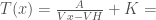
![{{[KV]x +[A -KVH]}\over {Vx - VH}}\,.](https://s0.wp.com/latex.php?latex=%7B%7B%5BKV%5Dx+%2B%5BA+-KVH%5D%7D%5Cover+%7BVx+-+VH%7D%7D%5C%2C.&bg=ffffff&fg=444444&s=0&c=20201002)
(Almost. We’re omitting the calculations concerning AD-BC from sheer bone-laziness [and a feeling that suchlike technicalities may drive students to sneak out of the room while my back is turned]. That C is nonzero is already implicit since the division by W in the beginning of our latest calculation already implies that V is nonzero [go ahead and leave if you feel you must].)
Part of the point here is that LF would seem to have been tailor-made for our consideration in 148. We went to a lot of trouble to develop the theory of Shifts and Scalings; here’s a subset of the Rational Functions (that we’re now trying to understand) obtained by applying these transformations to the simplest rational function of all (as usual, I “really” mean [what I’ve already called] the simplest one worthy of the name: the reciprocal). The result is an infinite collection of “next-simplest” cases. If everybody wasn’t in such an all-fired hurry (to “climb Calculus Mountain”, as an old sparring partner of mine was wont to say), one would more-or-less of course begin an exploration of, say, Graphing Rational Functions by looking in some detail at graphing these particular Rational Functions.
Having done so, the instructor would then be in a position to say things like, “Remember how the vertical asymptote of a Linear Fractional function at x = H [which came from shifting that of the reciprocal function] showed up in the ‘f-notation’ code as an x–minus–H? Because this is how you get a zero denominator in the rational function you’re examining? Well, this generalizes to rational functions generally; in f/g, if we can factor (the polynomial) g into linear factors, we can then ‘read off’ the vertical asymptotes for that function…”
(WordPress has just correctly typeset some “quotes ‘within’ quotes”. For every one of these, anyway in my copy, one pays the price of maybe about a dozen opening apostrophes being set wrongly. I’ve made some remarks about this punctuation disaster and will link ’em (see?), and omit this paragraph, as soon as I find ’em [and have the leisure, and the access].)
As an example of the advantages of considering the class LF carefully, consider the computations involved in calculating the inverse of a linear fractional function. For specificity, let 
No, wait. Now that we’re here, let’s first remark in passing on the remarkable fact that the functions of LF are invertible (by which I mean “have inverse functions” as opposed to mere inverse relations—every relation has one of those…)—and that one sees this (literally!) by considering the graph of the reciprocal and noticing that Shifts and Scalings preserve the property of being a one-to-one function. This means that a function that’s one-to-one (these are precisely the “invertible” functions as my students had bloodywell better know on Wednesday; the code ![[x_1 \not= x_2] \Rightarrow [f(x_1)\not=f(x_2)]](https://s0.wp.com/latex.php?latex=%5Bx_1+%5Cnot%3D+x_2%5D+%5CRightarrow+%5Bf%28x_1%29%5Cnot%3Df%28x_2%29%5D&bg=ffffff&fg=444444&s=0&c=20201002)
One is at this point actually pointing at a graph of 

And the point I’m making here (if any, as it seems to me) is that this “literal seeing” I was referring to a moment ago is at the same time an appeal to the imagination: our audience is being asked to spin up a movie in the YouTube of their imaginations and “see” the Shift or the Stretch in question dynamically. This is why one pulls one’s hands apart to suggest “stretching”, or seems to “grab” an invisible graph and “shift” it (or what have you). When the visual imagination is well-developed (as it isn’t in me very well at all), one tends to prefer to study continuous phenomena as opposed to discrete ones in one’s mathematical work (I’m a “discrete” man myself [as is obvious if the two other claims of this sentence so far are taken as true])… but every user of advanced mathematics has to develop at least some skill working with both types of these phenomena.
So. With our visual “proof” that RF consists of invertible functions in hand, let’s invert one.
Our technique—write x = f(y) (interchanging the “usual” roles for the variables) and solve for y—will then call for a new “trick”. (To elaborate on this. The other functions considered, ![[x \mapsto (3x + 1)^5]](https://s0.wp.com/latex.php?latex=%5Bx+%5Cmapsto+%283x+%2B+1%29%5E5%5D&bg=ffffff&fg=444444&s=0&c=20201002)
![[x \mapsto {{\root5\of{x} - 1}\over3}]](https://s0.wp.com/latex.php?latex=%5Bx+%5Cmapsto+%7B%7B%5Croot5%5Cof%7Bx%7D+-+1%7D%5Cover3%7D%5D&bg=ffffff&fg=444444&s=0&c=20201002)
Actually, it’s a pretty familiar trick, and I’ve never failed to present it at the board in any 148 equivalent up until now. Putting 


Having calculated the inverse for this Linear Fractional function (and checked it if we know what’s good for us; I’ve used [half of] this kind of check as an exam problem many times), we can confidently tackle the generic one; one arrives at the remarkable fact that
![[x \mapsto {{Ax+B}\over{Cx+D}}]^{-1} = [x \mapsto {{Dx - B}\over{-Cx +A}}]\,.](https://s0.wp.com/latex.php?latex=%5Bx+%5Cmapsto+%7B%7BAx%2BB%7D%5Cover%7BCx%2BD%7D%7D%5D%5E%7B-1%7D+%3D+%5Bx+%5Cmapsto+%7B%7BDx+-+B%7D%5Cover%7B-Cx+%2BA%7D%7D%5D%5C%2C.&bg=ffffff&fg=444444&s=0&c=20201002)
The most remarkable feature of this fact may be its striking resemblence to the inverse of a two-by-two invertible matrix; but one need not know about such calculations to see that the manipulations of the constants are easily memorized (“swap” the values in the upper left and lower right [the “main diagonal”] and change the sign of the other two). Students preparing for exams involving the prospect of some need to compute the inverse of a linear fractional function might then choose to memorize this fact in order to forgo the kind of calculation we demonstrated a few paragraphs ago. (There’ll be no such problem in my exams this quarter.)
One will of course wish to try this trick out: the inverse of 
But—and this will be last of all—what I find most exciting about the topic of Inverses of Rational Functions is that we can “compute” them visually by applying the graphing principles developed earlier in our course. For blogging purposes my graphing skills might as well be nonexistent, so this will be in outline. The graph of ![[x \mapsto {{Ax+B}\over{Cx+D}}]](https://s0.wp.com/latex.php?latex=%5Bx+%5Cmapsto+%7B%7BAx%2BB%7D%5Cover%7BCx%2BD%7D%7D%5D&bg=ffffff&fg=444444&s=0&c=20201002)


I’ve got to prepare for actual classes now; have a nice week.
-
1
Pingback on Sep 22nd, 2020 at 4:13 pm
[…] Bricks Without Straw compositions02/20/09 And Into The Black rational functions02/23/09 One Must Imagine Vlorbik Happy moebius transformations02/24/09 I Quit: A Clarification mathblogging considered […]
-
2
Pingback on Dec 14th, 2020 at 12:59 pm
[…] 02/18/09 Bricks Without Straw compositions 02/20/09 And Into The Black rational functions 02/23/09 One Must Imagine Vlorbik Happy moebius transformations 02/24/09 I Quit: A Clarification mathblogging considered […]

March 19, 2015 at 2:27 am
more broken internet. i’ll soon be altogether helpless thanks to the (newspeak) “upgrades” that eternally make every god damn thing harder and harder like harrison fucking bergeron oh dear god why didn’t i quit long ago i *hate* this.
May 5, 2015 at 1:29 pm
static.ow.ly/docs/needham_t_visual_complex_analysis_bhj.pdf
outstanding on mobius: tristan needham.